Building a Prediction Engine using Spark, Kudu, and Impala
April 12th, 2016
Why should your infrastructure maintain a linear growth pattern when your business scales up and down during the day based on natural human cycles? There is an obvious need to maintain a steady baseline infrastructure to keep the lights on for your business, but it can be very wasteful to run additional, unneeded compute resources while your customers are sleeping, or when your business is in a slow season. Conversely, how many times have you wished you had additional compute resources during your peak season, or when everyone runs queries on Monday morning to analyze last week’s data?
Allocating resources dynamically to demand level, versus steady state resource allocation, may sound daunting. Luckily, advances in scalable open source technologies have made the task simpler than you might think. In this post, I will walk you through a demo based on the Meetup.com streaming API to illustrate how to predict demand in order to adjust resource allocation.
We’ll aim to predict the volume of events for the next 10 minutes using a streaming regression model, and compare those results to a traditional batch prediction method. This prediction could then be used to dynamically scale compute resources, or for other business optimization. I will start out by describing how you would do the prediction through traditional batch processing methods using both Impala and Spark, and then finish by showing how to more dynamically predict usage by using Spark Streaming.
Of course, the starting point for any prediction is a freshly updated data feed for the historic volume for which I want to forecast future volume. In this case, I discovered that Meetup.com has a very nice data feed that can be used for demonstration purposes. You can read more about the API here, but all you need to know at this point is that it provides a steady stream of RSVP volume that we can use to predict future RSVP volume.
Architecture of the demo
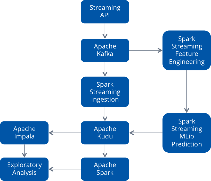
The basic architecture of the demo is to load events directly from the Meetup.com streaming API to Kafka, then use Spark Streaming to load the events from Kafka to Kudu. Using Kafka allows for reading the data again into a separate Spark Streaming Job, where we can do feature engineering and use MLlib for Streaming Prediction. The results from the predictions are then also stored in Kudu. We can also use Impala and/or Spark SQL to interactively query both actual events and the predicted events to create a batch forecast for comparison. See Figure 1 for an illustration of the demo.
You may wonder about my technology choices. Here’s a quick overview of why each is attractive for this challenge:
-
- Kafka allows me to abstract the data ingestion in a scalable way, versus tightly coupling it to the Spark streaming framework (which would have allowed only a single purpose). Kafka is attractive for its ability to scale to millions of events per second, and its ability to integrate well with many technologies like Spark Streaming.
- Spark Streaming is able to represent complex event processing workflows with very few lines of code (in this case using Scala, but it also allows for Java, Python, or R). It provides integration with Kafka and MLlib, the machine learning libraries within Spark.
- Apache Kudu does incremental inserts of the events. Its aim is to provide a hybrid storage layer between HDFS (leveraging its very fast scans of large datasets) and HBase (leveraging its fast primary key inserts/lookups). I could have chosen HBase or Cassandra for this, but Kudu can provide much faster scans of data for analytics, compliments of its columnar storage architecture.
- Impala enables us to easily analyze data that is being used in an ad-hoc manner. I used it as a query engine to directly query the data that I had loaded into Kudu to help understand the patterns I could use to build a model. As an alternative, I could have used Spark SQL exclusively, but I also wanted to compare building a regression model using the MADlib libraries in Impala to using Spark MLlib.
Building the demo
Now that I have explained the architecture choices, let’s jump into the process in more detail.
First, capture the stream to Kafka by curling it to a file, and then tailing the file to Kafka. This Github link contains the simple code for building this part of demo up through the Kafka load portion. And below, to give you some context of what the data looks like, is an example RSVP captured from the meetup.com stream:
{"response":"yes","member":{"member_name":"Richard
Williamson","photo":"http:\/\/photos3.meetupstatic.com\/photos\/member\/d\/a\/4\/0\/thu
mb_231595872.jpeg","member_id":29193652},"visibility":"public","event":
{"time":1424223000000,"event_url":"http:\/\/www.meetup.com\/Big-Data-
Science\/events\/217322312\/","event_id":"fbtgdlytdbbc","event_name":"Big Data Science
@Strata Conference,
2015"},"guests":0,"mtime":1424020205391,"rsvp_id":1536654666,"group":{"group_name":"Big
Data
Science","group_state":"CA","group_city":"Fremont","group_lat":37.52,"group_urlname":"Big-
Data-Science","group_id":3168962,"group_country":"us","group_topics":
[{"urlkey":"data-visualization","topic_name":"Data Visualization"},{"urlkey":"data-
mining","topic_name":"Data Mining"},{"urlkey":"businessintell","topic_name":"Business
Intelligence"},{"urlkey":"mapreduce","topic_name":"MapReduce"},
{"urlkey":"hadoop","topic_name":"Hadoop"},{"urlkey":"opensource","topic_name":"Open
Source"},{"urlkey":"r-project-for-statistical-computing","topic_name":"R Project for Statistical
Computing"},{"urlkey":"predictive-analytics","topic_name":"Predictive Analytics"},
{"urlkey":"cloud-computing","topic_name":"Cloud Computing"},{"urlkey":"big-
data","topic_name":"Big Data"},{"urlkey":"data-science","topic_name":"Data Science"},
{"urlkey":"data-analytics","topic_name":"Data Analytics"},
{"urlkey":"hbase","topic_name":"HBase"},
{"urlkey":"hive","topic_name":"Hive"}],"group_lon":-121.93},"venue":
{"lon":-121.889122,"venue_name":"San Jose Convention Center, Room
210AE","venue_id":21805972,"lat":37.330341}}
Once the Kafka setup is complete, load the data from Kafka into Kudu using Spark Streaming. We’re about to step through this code in more detail, but the full code can be found here.
The basic flow of the initial streaming ingest process involves first setting up the table in Kudu in a standard Spark job, and then running the Spark Streaming job to load the data to the table.
You can then create an external Impala table pointing to the Kudu data. This is done by running the schema in Impala that is shown in the Kudu web client for the table (copied here):
CREATE EXTERNAL TABLE `kudu_meetup_rsvps` (
`event_id` STRING,
`member_id` INT,
`rsvp_id` INT,
`event_name` STRING,
`event_url` STRING,
`TIME` BIGINT,
`guests` INT,
`member_name` STRING,
`facebook_identifier` STRING,
`linkedin_identifier` STRING,
`twitter_identifier` STRING,
`photo` STRING,
`mtime` BIGINT,
`response` STRING,
`lat` DOUBLE,
`lon` DOUBLE,
`venue_id` INT,
`venue_name` STRING,
`visibility` STRING
)
TBLPROPERTIES(
  'storage_handler' = 'com.cloudera.kudu.hive.KuduStorageHandler',
  'kudu.table_name' = 'kudu_meetup_rsvps',
  'kudu.master_addresses' = 'quickstart.cloudera:7051',
  'kudu.key_columns' = 'event_id, member_id, rsvp_id'
);
Then run a query against the above table in Impala, like this, to get the hourly RSVPs:
create
table   rsvps_by_hour as
select  from_unixtime(cast(mtime/1000 as bigint), "yyyy-MM-dd") as mdate
        ,cast(from_unixtime(cast(mtime/1000 as bigint), "HH") as int) as mhour
        ,count(*) as rsvp_cnt
from    kudu_meetup_rsvps
group
by      1,2
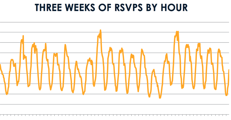
Once you have the RSVPs, plot them to show the pattern over time:
Next, do some simple feature engineering to later create a prediction model directly in Impala:
create
table rsvps_by_hr_training as
select
      case when mhour=0 then 1 else 0 end as hr0
      ,case when mhour=1 then 1 else 0 end as hr1
      ,case when mhour=2 then 1 else 0 end as hr2
      ,case when mhour=3 then 1 else 0 end as hr3
      ,case when mhour=4 then 1 else 0 end as hr4
      ,case when mhour=5 then 1 else 0 end as hr5
      ,case when mhour=6 then 1 else 0 end as hr6
      ,case when mhour=7 then 1 else 0 end as hr7
      ,case when mhour=8 then 1 else 0 end as hr8
      ,case when mhour=9 then 1 else 0 end as hr9
      ,case when mhour=10 then 1 else 0 end as hr10
      ,case when mhour=11 then 1 else 0 end as hr11
      ,case when mhour=12 then 1 else 0 end as hr12
      ,case when mhour=13 then 1 else 0 end as hr13
      ,case when mhour=14 then 1 else 0 end as hr14
      ,case when mhour=15 then 1 else 0 end as hr15
      ,case when mhour=16 then 1 else 0 end as hr16
      ,case when mhour=17 then 1 else 0 end as hr17
      ,case when mhour=18 then 1 else 0 end as hr18
      ,case when mhour=19 then 1 else 0 end as hr19
      ,case when mhour=20 then 1 else 0 end as hr20
      ,case when mhour=21 then 1 else 0 end as hr21
      ,case when mhour=22 then 1 else 0 end as hr22
      ,case when mhour=23 then 1 else 0 end as hr23
      ,case when mdate in ("2015-02-14","2015-02-15") then 1 else 0 end as weekend_day
      ,mdate
      ,mhour
      ,rsvp_cnt
from  rsvps_by_hour;
Install MADlib on Impala using this link, so that we can perform regression directly in Impala.
With the data loaded in Impala and the MADlib libraries installed, we can now build a simple regression model to predict hourly sales in an ad hoc manner.
The first step is to train the regression model as follows:
select  printarray(linr(toarray(hr0,hr1,hr2,hr3,hr4,hr5,hr6,hr7,hr8,hr9,hr10,hr11,hr12,hr13,hr14, hr15,hr16,hr17,hr18,hr19,hr20,hr21,hr22,hr23,weekend_day), rsvp_cnt))
from    rsvps_by_hr_training;
This gives us the following regression coefficients. Looking at these, you can see that the first 24 coefficients show a general hourly trend with larger values during the day, and smaller values during the night, when fewer people are online. The last coefficient corresponding to the weekend indicator shows that, if it is a weekend day, then volume is reduced due to the negative coefficient—which is what we expect by looking at the data:
| Feature | Coefficient |
| hr0 | 8037.43 |
| hr1 | 7883.93 |
| hr2 | 7007.68 |
| hr3 | 6851.91 |
| hr4 | 6307.91 |
| hr5 | 5468.24 |
| hr6 | 4792.58 |
| hr7 | 4336.91 |
| hr8 | 4330.24 |
| hr9 | 4360.91 |
| hr10 | 4373.24 |
| hr11 | 4711.58 |
| hr12 | 5649.91 |
| hr13 | 6752.24 |
| hr14 | 8056.24 |
| hr15 | 9042.58 |
| hr16 | 9761.37 |
| hr17 | 10205.9 |
| hr18 | 10365.6 |
| hr19 | 10048.6 |
| hr20 | 9946.12 |
| hr21 | 9538.87 |
| hr22 | 9984.37 |
| hr23 | 9115.12 |
| weekend_day | -2323.73 |
Now we can apply the above coefficients to future data to predict future volume. In production we would have written the coefficients to a table as done in the MADlib blog post we used above, but for demo purposes we just substitute them as follows:
select       mdate,
             mhour,
             cast(linrpredict(toarray(8037.43, 7883.93, 7007.68, 6851.91, 6307.91, 5468.24, 4792.58, 4336.91, 4330.24, 4360.91, 4373.24, 4711.58, 5649.91, 6752.24, 8056.24, 9042.58, 9761.37, 10205.9, 10365.6, 10048.6, 9946.12, 9538.87, 9984.37, 9115.12, -2323.73), toarray(hr0, hr1, hr2, hr3, hr4, hr5, hr6, hr7, hr8, hr9, hr10, hr11, hr12, hr13, hr14, hr15, hr16, hr17, hr18, hr19, hr20, hr21, hr22, hr23, weekend_day)) as int) as rsvp_cnt_pred,
             rsvp_cnt
from         rsvps_by_hr_testing
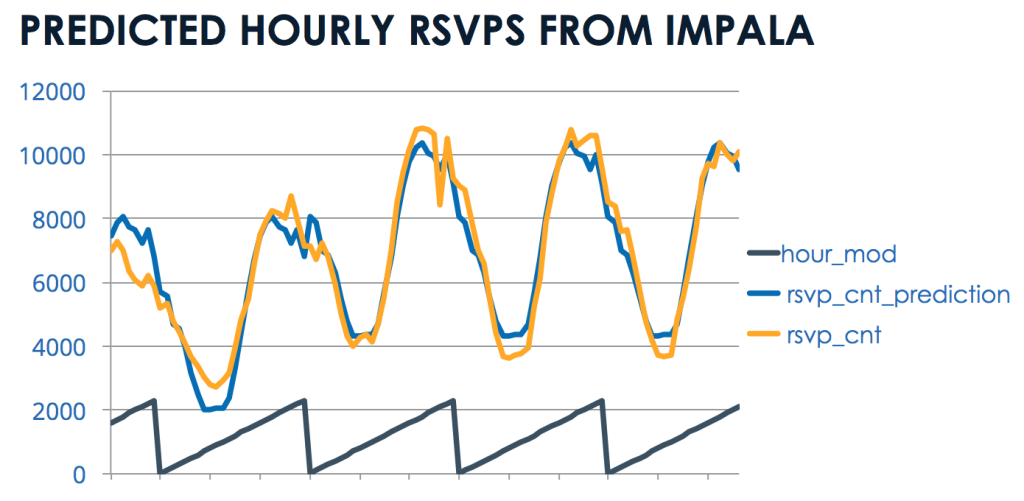
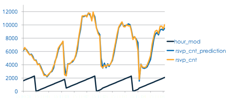
Figure 3 shows how the prediction looks compared to the actual RSVP counts with hour mod, just helping to show the time-of-day cycle. (Due to limited data, the last couple of days of the time range were withheld from training for this example.)
Using a Spark Model Instead of an Impala Model
Now let’s look at how to build a similar model in Spark using MLlib, which has become a more popular alternative for model building on large datasets.
First, load the json file into Spark and register it as a table in Spark SQL. You could load from Kudu too, but this example better illustrates that Spark can also read the json file directly:
val path = "/home/demo/meetupstream1M.json"
val meetup = sqlContext.read.json(path)
meetup.registerTempTable("meetup")
You then run a similar query to the one we ran in Impala in the previous section to get the hourly RSVPs:
val meetup2 = sqlContext.sql("
   select from_unixtime(cast(mtime/1000 as bigint), 'yyyy-MM-dd') as dy,
          case when from_unixtime(cast(mtime/1000 as bigint),'yyyy-MM-dd') in ('2015-02-14','2015-02-15') then 1 else 0 end as weekend_day,
          from_unixtime(cast(mtime/1000 as bigint), 'HH') as hr,
          count(*) as rsvp_cnt
    from  meetup
    where from_unixtime(cast(mtime/1000 as bigint), 'yyyy-MM-dd') >= '2015-10-30'
    group
    by    from_unixtime(cast(mtime/1000 as bigint), 'yyyy-MM-dd'),
          from_unixtime(cast(mtime/1000 as bigint), 'HH')")
With that done, you can move to the next transformation step: creating feature vectors. There was a time when you’d have to do the same feature engineering in the verbose query above (with case statements) to accomplish this. However, my colleague Andrew Ray’s recent Spark contributions have fixed this. You can now just run the following one-liner to pivot the data into the needed feature vectors:
val meetup3 = meetup2.groupBy("dy","weekend_day","hr","rsvp_cnt").pivot("hr").count().orderBy("dy")
Now that you have the data in the basic structure that we are looking for, you can train a similar regression model to the one we did in Impala, as follows:
import org.apache.spark.mllib.regression.RidgeRegressionWithSGD
import org.apache.spark.mllib.linalg.Vectors
import org.apache.spark.mllib.regression.LabeledPoint
val trainingData = meetup3.map { row =>
      val features = Array[Double](1.0,row(1).toString().toDouble,row(4).toString().toDouble,
                                   row(5).toString().toDouble,row(6).toString().toDouble,
                                   row(7).toString().toDouble,row(8).toString().toDouble,
                                   row(9).toString().toDouble,row(10).toString().toDouble,
                                   row(11).toString().toDouble,row(12).toString().toDouble,
                                   row(13).toString().toDouble,row(14).toString().toDouble,
                                   row(15).toString().toDouble,row(16).toString().toDouble,
                                   row(17).toString().toDouble,row(18).toString().toDouble,
                                   row(19).toString().toDouble,row(20).toString().toDouble,
                                   row(21).toString().toDouble,row(22).toString().toDouble,
                                   row(23).toString().toDouble,row(24).toString().toDouble,
                                   row(25).toString().toDouble,row(26).toString().toDouble,
                                   row(27).toString().toDouble)
      LabeledPoint(row(3).toString().toDouble, Vectors.dense(features))
}
trainingData.cache()

val model = new RidgeRegressionWithSGD().run(trainingData)
And then score a new set of data as follows (just scoring same data set for illustration here):
val scores = meetup3.map { row =>
      val features = Vectors.dense(Array[Double](1.0,row(1).toString().toDouble,
                                                 row(4).toString().toDouble,row(5).toString().toDouble,
                                                 row(6).toString().toDouble,row(7).toString().toDouble,
                                                 row(8).toString().toDouble,row(9).toString().toDouble,
                                                 row(10).toString().toDouble,row(11).toString().toDouble,
                                                 row(12).toString().toDouble,row(13).toString().toDouble,
                                                 row(14).toString().toDouble,row(15).toString().toDouble,
                                                 row(16).toString().toDouble,row(17).toString().toDouble,
                                                 row(18).toString().toDouble,row(19).toString().toDouble,
                                                 row(20).toString().toDouble,row(21).toString().toDouble,
                                                 row(22).toString().toDouble,row(23).toString().toDouble,
                                                 row(24).toString().toDouble,row(25).toString().toDouble,
                                                 row(26).toString().toDouble,row(27).toString().toDouble))
      (row(0),row(2),row(3), model.predict(features))
}

scores.foreach(println)
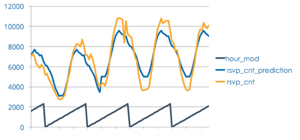
Figure 4 shows how the Spark model results compare to actual RSVP counts (with the same withholding period as we used in Impala):
Using a Spark Streaming Regression Model
The last two examples (Impala MADlib and Spark MLlib) showed us how we could build models in more of a batch or ad hoc fashion; now let’s look at the code to build a Spark Streaming Regression Model. Using a streaming approach to model building allows us to update the model in a much more frequent manner, in order to benefit from the most recent data available — thus hopefully improving accuracy.
Here, we’ll take a bit of a different approach compared to the batch predictions done above. In order to illustrate using the streaming regression model, we simply use the count of RSVPs per minute (instead of by hour when doing prior batch predictions) as a way to easily generate a continuous streaming forecast of what the next 10 minutes will hold in the way of RSVPs.
To do this, first setup the stream ingestion from Kafka (excerpts below are from the full code in GitHub).
This part of the code simply sets up the Kafka stream as our data input feed. It takes the Kafka topic, broker list (Kafka server list) and the Spark Streaming context as input parameters. It then gets a connection to Kafka to subscribe to the given topic, and ingest the data into the stream processing flow.
     def loadDataFromKafka(topics: String,
                           brokerList: String,
                           ssc: StreamingContext): DStream[String] = {
            val topicsSet = topics.split(",").toSet
            val kafkaParams = Map[String, String]("metadata.broker.list" -> brokerList)
            val messages = KafkaUtils.createDirectStream[String, String, StringDecoder, StringDecoder](ssc, kafkaParams, topicsSet)
            messages.map(_._2)
     }

     val dstream = loadDataFromKafka(topics, brokerList, ssc)
Transform the stream to RSVP counts by minute using SQL inside the stream. Do this by reading the json stream:
     val stream = dstream.transform { rdd =>
     val parsed1 = sqlContext.read.json(rdd)
     parsed1.registerTempTable("parsed1")
     val parsed2 = sqlContext.sql("
            select  m,
                    cnt,
                    mtime
            from    (select   (round(mtime/60000)-(" + current_time + "/60000 ))/1000.0 as m,
                              count(*) as cnt,
                              round(mtime/60000) as mtime
                    from      (select distinct * from parsed1) a
                    group
                    by        (round(mtime/60000)-(" + current_time + "/60000 ))/1000.0,
                              round(mtime/60000) ) aa
            where   cnt > 20
            ")
     parsed2.rdd
     }
     stream.print()
The SQL above converts the mtime into m (a derived variable we can use to understand the linear increase in time) by calculating the nbr of minutes from the current time and then dividing it by 1000 — to make the scale smaller for the regression model — and then counting the nbr of RSVPs for each minute (subsetting on minutes with at least 20 RSVPs in order to exclude non-relevant time periods that trickle in late; this would be done more robustly in production, subsetting on time period instead).
After this transformation, set up the data structures for modeling: one stream for training data, actl_stream, and one stream for predictions, pred_stream. For the prediction stream, just build the next set of 10-minute time intervals from the current training interval (this would be done differently for production by just building a fixed stream of future time from the current time, but works well for illustration):
     val actl_stream = stream.map(x =>
           LabeledPoint(x(1).toString.toDouble,Vectors.dense(Array(1.0,x(0).toString.toDouble))) ).cache()
     actl_stream.print()
     val pred_stream = stream.map(x =>
           LabeledPoint((x(2).toString.toDouble+10)*60000,Vectors.dense(Array(1.0,x(0).toString.toDouble))) )
     pred_stream.print()
Now we are ready to train the streaming model using the time interval as a trend feature, and the RSVP counts by minute as the historic volume feature. This is a very simple starting point for the streaming model, mainly for simple illustration purposes. A full production model would also incorporate the features I discussed earlier, including hour-of-day and weekday, as well as other features to improve the forecast accuracy.
     val numFeatures = 2
     val model = new StreamingLinearRegressionWithSGD().setInitialWeights(Vectors.zeros(numFeatures)
     model.trainOn(actl_stream)
Finally, apply the prediction model to the future time intervals to come up with the predictions:
     val rslt_stream = model.predictOnValues(pred_stream.map(lp => (lp.label, lp.features)))
     rslt_stream.print()
Figure 5 shows the plotted results of the streaming model on a similar dataset. (This was for a future week of data, as the streaming model was developed after original non-streaming models.)
As you can see, given that we are now taking advantage of the most recent 10 minutes of RSVP activity, we can generate a much better forecast than the prior methods for the next 10 minutes. However, in order to make the forecast even better, future steps would be taken to combine additional features into the streaming forecast to improve the robustness of the model. Also, now that the predictions are being streamed into Kudu, it would be very easy to build an API so as to use the predictions to begin adjusting resources to adapt to the demand.
I encourage you to try this method in your own work, and let me know how it goes. I look forward to hearing about any challenges I didn’t note, or improvements that could be made.


